
Model checking - A short informal Introduction
The essential concept behind model checking is to (mathematically) prove whether a given model (a set of system requirements or a simulation
model) satisfies a certain specification property.
Sometimes a more formal definition can be found:
Given a model M and a formula φ, model checking is the problem of verifying whether or not φ is true in
M.
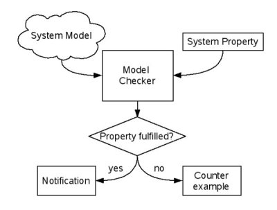
A typical model checking work-flow
As shown in the Figure above, traditional model checking is composed of three major steps:
- Define a formal model of the system that is subject to verification by creating a model of the system in a language that fits the model checker's input language. Those modeling languages are usually tight coupled to the model checker itself, like the PROMELA language of the SPIN model checker.
- Provide a particular system property that should be proved. In other words, a question about the system's behavior is formulated that should be answered by the model checker.
- Invoke the model checking tool and receive a notification whether the given system property was fulfilled or not. In case the system property could not be verified, a counterexample is generated to finger-point to the source of error in the simulation model.
"Model checking is an automatic, model-based, property verification approach."
Using Kripke structures to represent a system's behavior
In model checking, finite (nondeterministic) state machines are used to represent the behavior of the system. A special type of these state
machines are Kripke structures. Every single state is labeled with boolean variables
(atomic propositions), which are the evaluations of expressions in that state. These expressions correlate to the particular system properties,
e.g. boolean expressions over variables or registers.
A Kripke structure M is represented as an ordered sequence of four objects:
M = (S, s0, R, L)
S: finite set of states
s0: initial state
R: transition relation
L: interpretation function
The transition relation specifies for each state whether and which successor states are possible.
The interpretation function labels each state with the set of atomic propositions that are true in that state.
Coffee vending machine example:
A simple coffee vending machine model is introduced to demonstrate a possible application of Kripke structures. It's textual functional description reads as follows:
- After inserting a coin, the user can choose her/his favorite coffee.
- A coffee is only brewed after a valid selection is made.
- The user is able to abort the procedure at any time.
The following Figure shows the resulting Kripke structure, with all the states, transitions and state variables.
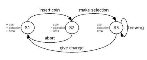
The coffee vending machine Kripke structure
From transition systems towards to computation paths
By simply unwinding the Kripke structure it is possible to visualize all computation paths:
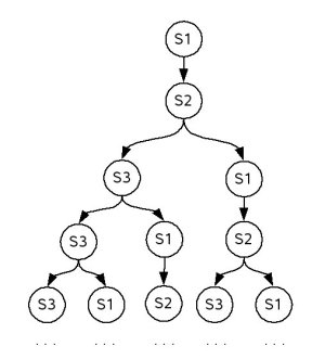
The first few computation paths of the coffee vending machine example
CTL at a glance
Model checking is based on mainly temporal logic. One main representative is CTL (Computation Tree Logic). CTL is a combination of a linear temporal logic and a
branching-time logic and was introduced by Clarke & Emerson in 1980.
In a linear temporal logic, various operators are provided to describe events along a single computation path. In contrary, a branching-time
logic provides operators to quantify over a set of states that are successors of a given (the current) state. CTL combines these two kinds of
operators.
CTL Syntax
Each CTL operator consists of two symbols. The first one is either A (which stands for All paths), or E (there Exists a path). The second one is either X (the neXt state), F (in Future state), G (Globally in the future) or U (Until). A and E are path quantifiers, X, F, G and U are linear-time operators.
Expressing a CTL system property for the coffee vending machine example
For the coffee vending machine some conceivable system properties could be:
(1) In spoken language: A coffee is brewed after a selection was made.
In CTL syntax this would result in: E[(¬ selection) U (brew)] ... As long as no selection was made, no coffee is brewed in any cases. After a selection is made, coffee is brewed for sure.
(2) In spoken language: A coffee is brewed in any case.
In CTL syntax this would result in: AG[(brew)] ... Coffee will be brewed from now on, no matter what happens.
State Space Explosion
Kripke structures can become large and complex for real life systems. The logical consequence is, that the state
space of such a system is tremendous too, or even infinite. Hence, without any optimizations of the state space, it is impossible for most of the
applications to explore the entire state space, since time and memory are limited.
If model checking should be performed on a typical embedded system a variety of components can result in a state space multiplication. Suppose
that the embedded system uses an n-bit ADC to read environment variables. Every time the ADC value is read, state space is expanded by
2n. For a 16-bit wide ADC this would result in adding additional 65536 paths. The next Figure visualizes such a transition.
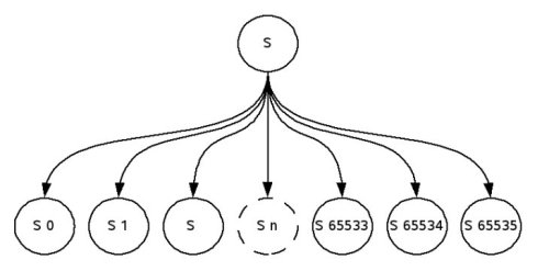
State Space Explosion after reading ADC values